While working on LGS, the programmers at LEDAS developed similar software for Dassault Systèmes, which were integrated into CATIA and so are used by hundreds of thousands engineers in corporations like Toyota, Honda, Airbus, and Boeing. Much later, LEDAS was asked to develop constraint solvers that met specific requirements, in addition to long-term projects we already had fulfilled with two other customers.
To illustrate the importance of the geometric constraint solver, let's look at some of the design tasks that require it. The word "design" has at least two meanings: either graphic design or engineering design. While graphic designers tend to make drawings freehand, engineers need to create shapes that are precise, with predetermined relationships and properties.
The typical task of design engineers is to create 3D models of mechanisms consisting of parts precisely positioned with respect to one other. The positioning is defined by geometric constraints. Constraints force parts to be parallel to each other, be located at specific distances or angles, to touch one another, be concentric, and so on. To create assemblies of parts, it is necessary to solve the systems of constraints. This is what a geometric solver is for.
Given a system of constraints, the geometric solver works through systems of nonlinear algebraic and trigonometric equations to arrive at a feasible solution, and then applies spatial transformations to each part in the assembly. As a result, every detail is placed in a position that satisfies all required constraints.
Since their development in the early 2000s, the solving of nonlinear systems has become a well-used task in computational mathematics. In practice, however, systems of equations derived from geometric constraints in CAD might be very specific. They can have problems, such as being underdefined, overdefined, they also can be sparse. Let’s look at what each of these mean.
A sequence of underdefined models in the design process
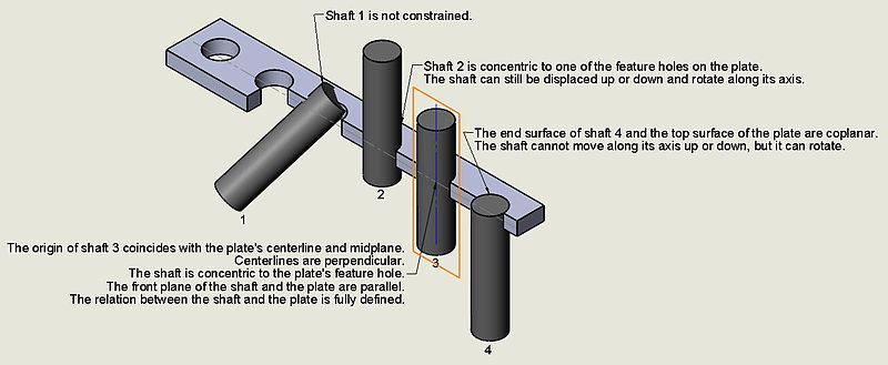
Underdefined. In most cases, systems of equations are underdefined. Here’s how. Each three-dimensional part has six degrees of freedom (six ways to move): three translational (moving in the three dimensions of x, y, and z) and three rotational (rotating about the three axes). An engineer sets some constraints to fix certain degrees of freedom, and leaves the remaining ones free to move, as required by the mechanism. This is an example of an underdefined system. It results in an infinite number of possible solutions, from which the geometric solver must choose one that places the parts as close to the initial positions as possible.
Overdefined. On the other hand, the system of equations can be overdetermined when for example, you take as a simple model a house made of wooden boards, and then apply parallel and perpendicular constraints to all pairs of boards. In practice, some parallelisms and perpendicularities follow from others, and so are not needed. This means that in the system of equations there will be dependencies that lead to serious problems.
In another example, the data in the original model might be inaccurate (maybe, because of accumulation of rounding errors on previous steps of modeling), from which the linearly dependent equations may become not linearly dependant, although, strictly speaking, they should be dependant. As a result, the condition number of the system of equations increases sharply, the calculations become unstable, and a convergence is no longer possible.
Yet another example of overdefined (but consistent) constraint system
Sparse. The third case is sparseness of constraint systems. As a rule, one constraint applies to only two objects, such as, for example, making two cylinders concentric. This sparseness means that the system of nonlinear equations can be divided into weakly connected subsystems, which makes it possible to use special decomposition methods formulated both in algebraic and geometric form.
Of course, to implement a real-world industrial-strength constraint solver you need to be able to do a lot of difficult things, including:
- Decompose the problem into parts
- Solve differential equations to move and rotate objects, while keeping constraints satisfied
- Support black-box and white-box curves and surfaces
- Avoid singularities and bifurcation points, and many other things.