Geometric modelling is typically based on numerical methods that calculate derivatives of functions.
One significant example is constraint solving, which involves solving systems of non-linear equations. Popular classes of numerical methods, like the Newton Method, are based on calculating the Jacobian matrix for a system, i.e., the values of partial derivatives of each equation's expression by each of the variables of the system.
Another fundamental use case is calculating the intersecting curve between two surfaces in 3D space. This is reduced to solving a small system of three non-linear equations with four variables – two parameters of each of the two surfaces.
Both these examples illustrate the fact that the functions we need to differentiate can be quite complex and diverse: different geometric constraints and types of surfaces might lead to different expressions based on basic operations (summation, multiplication, etc.) as well trigonometric functions (sin, atan and etc).
So, the developers of geometric modelling algorithms face the problem of implementing expressions of derivatives in modelling functions, along with the function itself. For a single function, a valid way to perform the derivatives function calculation would be doing it "on a piece of paper" and then turning the program directly into code:
def f(x, y):
    val = x * sin(y)
    dfdx = sin(y)
    dfdy = x * cos(y)
    return (val, (dfdx, dfdy))
This approach, however, leaves responsibility for matching the function expression and the expressions of its derivatives to the developer. When support for many such functions is required (such as modelling different types of constraints, or intersecting different types of surfaces), this "manual differentiation" approach puts a significant maintenance load on the code. We are forced to implement n+1 complicated expressions for n-variable functions, instead of a single expression, even when we need just a first-order partial derivative. Also, we need to manually (or with a series of unit tests) check the correctness of the derivative expressions, to ensure they actually match the expressions of the functions, being the calculation for the corresponding derivatives.
It is worth mentioning that mistakes in this kind of correspondence between functions and their derivative expressions might be really hard to find. Usually, these numerical methods lead to a reduced chance of convergence and lowered speed of convergence. However, properly implemented numeric methods can still fail to converge or else converge too slowly from certain start points, and so it is not always possible. Problems of convergence can be caused by the nature of the function and its convergence areas for certain methods, or by mistakes in the derivatives expressions themselves.
Manually implemented derivative expressions could potentially become problematic parts of the code. This is a burden we’d be happy to be rid of.
So, not surprisingly, developers are very much interested in how to calculate derivatives automatically, rather than implement their own. Let’s consider three ways of performing differentiation: symbolic, numeric, and forward accumulation.
Symbolic Differentiation
Symbolic differentiation is the closest method to how graduates of mathematics would approach differentiation. It reminds me of the way we did differentiation in our calculus courses.
Being an explicit form of an expression for function evaluation, symbolic differentiation builds explicit expressions for the derivative as independent objects. Then, we query it at any point, independently of the parent function, as the following code illustrates:
    from sympy import symbols, diff, sin
    x, y = symbols('x y')
    f = x * sin(y)
    f_x = diff(f, x)
    f_y = diff(f, y)
    print("{0}, {1}".format(f_x, f_y))

    Output:
    sin(y), x*cos(y)
To better understand the pros and cons of this approach, let’s consider its "opposite alternative," the numeric calculation of derivatives.
Numeric Differentiation
Numeric differentiation comes from another branch of mathematics -- numeric methods. In effect, it calculates approximations to derivatives at certain points, rather than exact values. It works like this:
def firstDeriv(func, vars, idx, h):
    left = vars
    left[idx] = vars[idx] - h
    right = vars
    right[idx] = vars[idx] + h
    return (func(right) - func(left)) / (2 * h)
There are several formulas for numeric differentiation, providing different guaranteed approximations. For example, the one I implemented above is known as the "symmetric difference" method:
f'(x) = (f(x+h) – f(x–h))/2h
It provides O(h2) estimation, i.e., the guaranteed deviation of the calculated expression.
Now let’s turn to the pros and cons. The key feature of numeric differentiation is that it is the simplest way to implement code, as shown above. It works universally with all "black box" functions (i.e. functions without explicit expression built from analytic primitives, but literally any object returning some value for any set of input variable values).
The cons, in turn, are preciseness and performance. As stated, the numeric method gives an approximation to the mathematical value of derivative, having, e.g. an asymptotics of O(h2) for symmetric differences. On the other hand, subtraction of two big numbers to get a smaller one, and then division by another small number, produces rounding errors. These errors are estimated as O(ε/h), where is a double precision constant of order 10-16.
The optimal h for minimizing the maximum of these two errors lies at h≈10-4. For example, see below the graph of absolute errors for the value of (x*lnx)'(e). They are calculated with the symmetric difference formula for different values of step h.
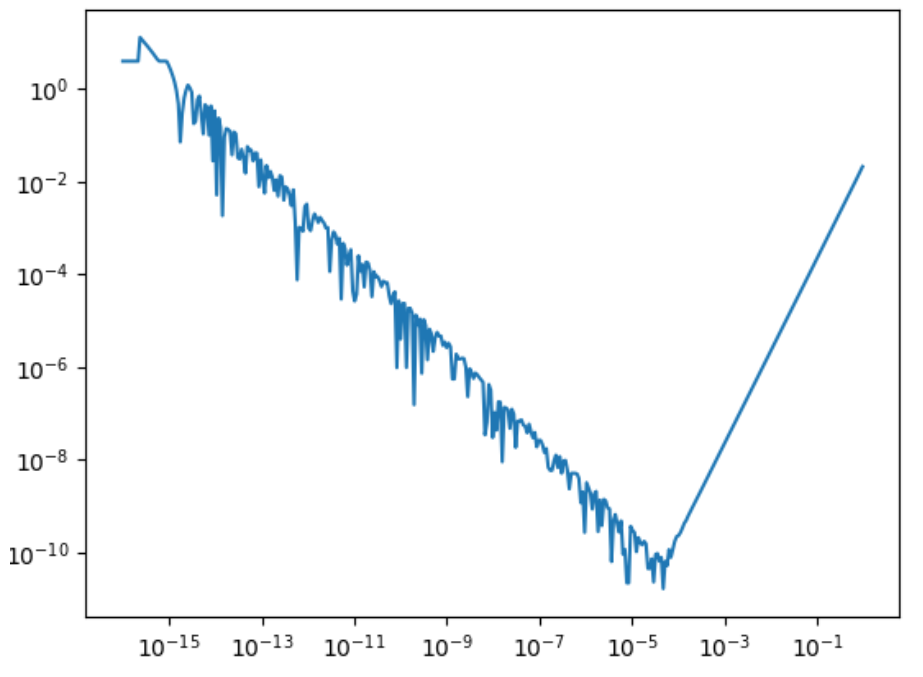
The best attained precision of ≈10-11 can potentially slow down derivative-based numeric methods, compared to more precisely calculated derivatives, as well as limit the overall convergence precision.
The pros and cons for symbolic differentiation are reversed from numeric differentiation. The implementation is much more complex, requiring representations of the function as a tree of atomic operations, each of them implementing a differentiation formula that builds subtrees for derivatives.
For example, multiplication node mult(left, right) would construct a derivative subtree as deriv(mult)=plus(muilt(left,deriv(right),mult(right,deriv(left)) according to the corresponding mathematical formula.
Obtaining an expression tree for derivatives is often more complex than an expression tree of the function itself. Evaluation along the tree could, however, be faster than a double evaluation of the initial expression required to calculate the derivative numerically.
In terms of performance, there is an initial overhead during the building of derivative expressions. So, the performance gain is achieved only when doing multiple evaluations, which is the case in numeric solving methods. The construction overhead can be potentially eliminated from the running time by moving it to the compile time using code generation utilities.
Forward Accumulation
The forward accumulation approach (also called "automatic differentiation" by some sources) stands between numeric and symbolic differentiations, and attempts to provide the advantages of both.
In essence, it is similar to symbolic differentiation, but without the explicit construction of derivative expressions. Instead, it is calculated on the fly, along a function expression tree. Overloaded atomic operations (like the mult binary operation from the example above, or basic analytic functions like sine, natural logarithm, and so on) are overloaded to calculate both the value and the derivative(s) according to basic differentiation formulas.
It can be seen as representing functions like a Taylor series truncated to the required order of differentiation, and implementing operations on corresponding polynomes:
class Taylor:
    val = 0
    derivs = ()
    def __init__(self, iVal, iDerivs):
        self.val = iVal
        self.derivs = iDerivs

    def __add__(self, other):
        self.val += other.val
        self.derivs = tuple(map(lambda x, y: x + y, self.derivs, other.derivs))
        return self

    def __mul__(self, other):
        if (isinstance(other, int) or isinstance(other, float)):
            self.derivs = tuple(map(lambda x: other * x, self.derivs))
            self.val *= other
        else:
            self.derivs = tuple(map(lambda x, y: other.val * x + self.val * y, self.derivs, other.derivs))
            self.val *= other.val
        return self

def f(x, y):
    return x * x + y * 4

x = Taylor(5, (1, 0))
y = Taylor(7, (0, 1))
fe = f(x, y)
print(fe.val, fe.derivs)
This method is simpler in implementation, but retains all the advantages of symbolic differentiation, including precision and calculation time.
Blackbox sub-expressions can be embedded into this scheme by directly assigning the value and derivatives vector to some sub-expression. This partially eliminates the remaining disadvantage of working with explicit expressions constructed from atomic expressions, and allows us to incorporate pure blackbox functions in our calculation schemes.
Conclusion
I highly recommend using the forward accumulation (automatic differentiation) approach in numeric algorithms. It adds simplicity to developers’ work in finding and implementing a variety of modelling approaches, relieving them from having to calculate and implement derivative expressions manually. It increases the stability of the algorithms, and eliminates hard-to-find mistakes from mismatches between functions and derivative expressions.
According to our experience, forward differentiation tends most often to become the tool of choice, as it combines relative simplicity of implementation with precise calculations.